POLS 1600
Causal Inference in
Experimental Designs
Updated Apr 22, 2025
Setting your working directory when working “Live”

Practice
- Create two variables
xandyxshould be a random variable with 100 observations from a random normal (rnorm) distribution with mean 0 and standard deviation 1yshould be a function of x plus the square of a random normal distribution with mean 0 and standard deviation 1
- Combine
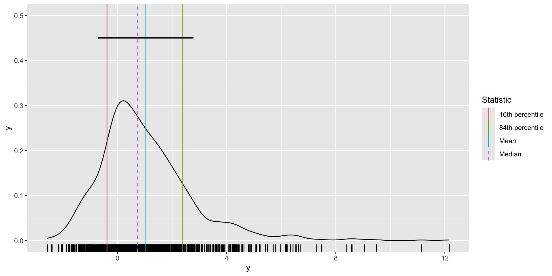
xandyinto adata.framecalleddf summarizethemean,median, standard deviation (sd), 16th and 84th percentile (quantile) ofxandyand save this to an object calleddf_sum- Plot the distributions of
xandy, separately, using a density plot (geom_density)- Add a rug to each density plot
- Add vertical lines for the mean and median of each variable
- A vertical lines at the 16th and and 84th percentile of each plot
- Hint: use your object
df_sumas the data for these geometries
- Hint: use your object
# Load libraries
library(tidyverse)

# Set seed for reproducibility
set.seed(123)

# Number of observations
n <- 1000

# Generate data
x <- rnorm(n, mean = 0, sd = 1)
y <- x + (rnorm(n, mean = 0, sd = 1))^2

# Create dataframe
df <- data.frame(x = x, y = y)

# Calculate summary statistics

df_sum <- df %>%
  dplyr::summarise(
    x_mean = mean(x),
    x_median = median(x),
    x_sd = sd(x),
    x_16th = quantile(x, probs = .16),
    x_84th = quantile(x, probs = .84),
    y_mean = mean(y),
    y_median = median(y),
    y_sd = sd(y),
    y_16th = quantile(y, probs = .16),
    y_84th = quantile(y, probs = .84)
  )

df_sum
x_mean x_median x_sd x_16th x_84th y_mean y_median
1 0.01612787 0.009209639 0.991695 -1.01607 0.9869428 1.036354 0.7302196
y_sd y_16th y_84th
1 1.738673 -0.3879478 2.390059fig_x <- df %>%
ggplot(aes(x))+
geom_density()+
geom_rug()+
geom_vline(
data = df_sum,
aes(xintercept = x_mean, col="Mean"))+
geom_vline(
data = df_sum,
aes(xintercept = x_median, col="Median"),
linetype = "dashed")+
geom_vline(
data = df_sum,
aes(xintercept = x_16th, col="16th percentile"))+
geom_vline(
data = df_sum,
aes(xintercept = x_84th, col="84th percentile"))+
geom_segment(
aes(y=.45, yend=.45,
x = df_sum$x_mean - df_sum$x_sd,
xend = df_sum$x_mean + df_sum$x_sd)
)+
ylim(0,.5)+
labs(
col = "Statistic"
)
fig_y <- df %>%
ggplot(aes(y))+
geom_density()+
geom_rug()+
geom_vline(
data = df_sum,
aes(xintercept = y_mean, col="Mean"))+
geom_vline(
data = df_sum,
aes(xintercept = y_median, col="Median"),
linetype = "dashed")+
geom_vline(
data = df_sum,
aes(xintercept = y_16th, col="16th percentile"))+
geom_vline(
data = df_sum,
aes(xintercept = y_84th, col="84th percentile"))+
geom_segment(
aes(y=.45, yend=.45,
x = df_sum$y_mean - df_sum$y_sd,
xend = df_sum$y_mean + df_sum$y_sd)
)+
ylim(0,.5)+
labs(
col = "Statistic"
)
cor(df$x, df$y)[1] 0.5779469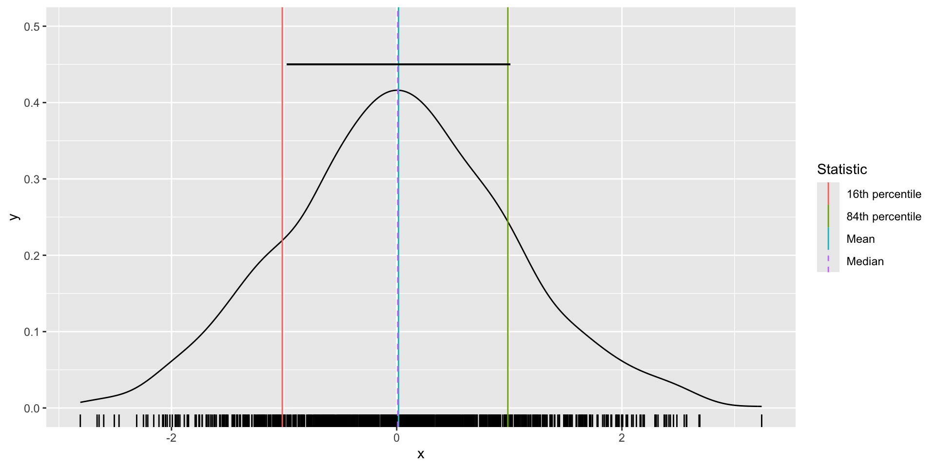

Measures of central tendency describe what’s typical
Measures of dispersion describe variation around what’s typical
Causal claims imply counterfactual comparisons
Causal claims imply counterfactual comparisons
What would have happened if we were to change some aspect of the world?

Casual claims are all around us


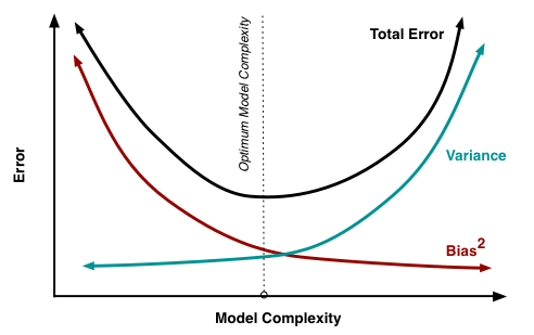
Bias vs. variance
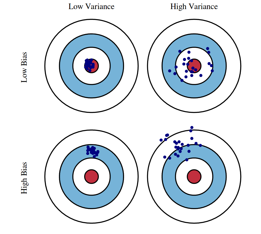
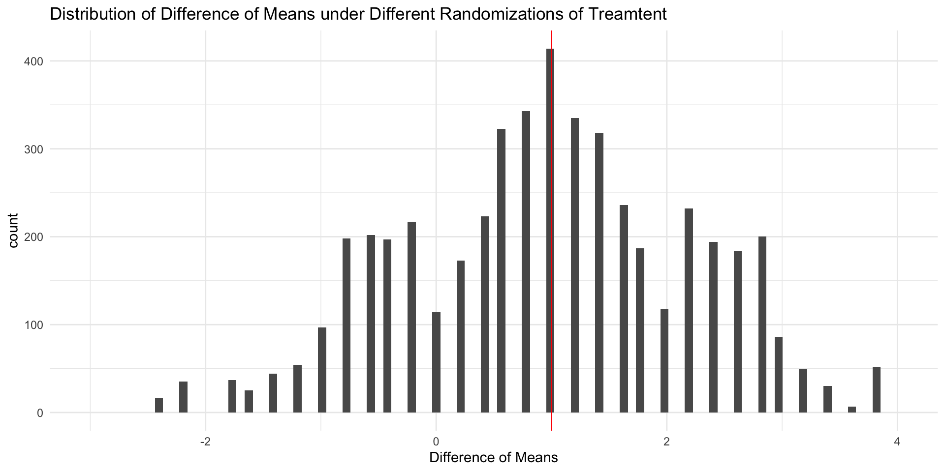
The bias-variance tradeoff
Distribution of Sample ATEs