POLS 1600

Probability:
Distributions and Limit Theorems

Updated May 31, 2024

Overview

Class Plan

  • Announcements (5 min)
  • Feedback (5 min)
  • Class plan
    • Probability Distributions (20 min)
    • Law of Large Numbers (20 min)
    • Central Limit Theorem (20 min)
    • Standard Errors (10 min)

Goals

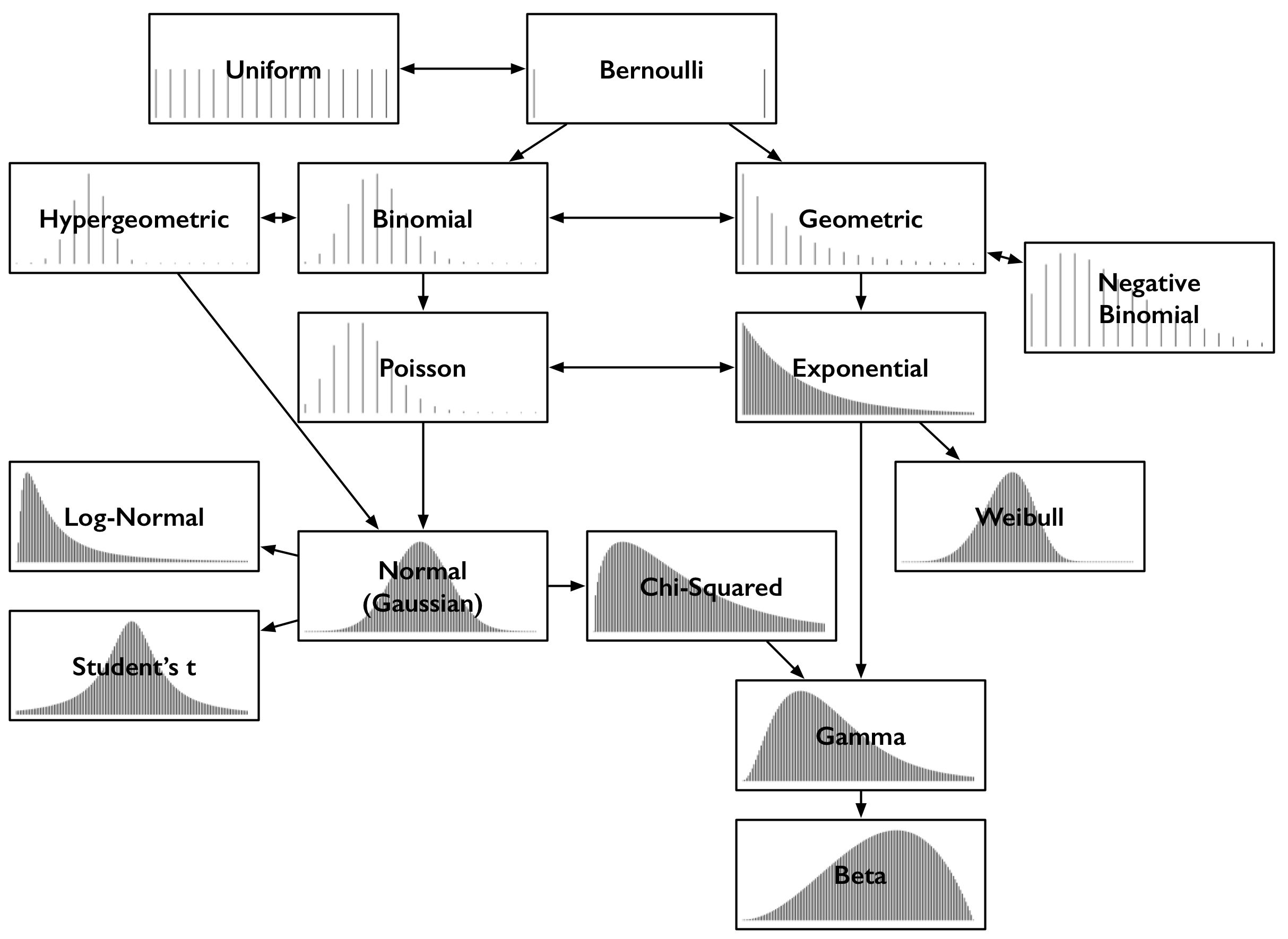
  • Probability distributions allow us to describe different data generating processes and quantify uncertainty about estimates

  • The Law of Large Numbers tells us that the mean of a sample converges to the mean of population as the size of the sample grows larger.

  • The Central Limit Theorem tells us that distribution of sample means of a given sample size converges in distribution to a Normal probability distribution

  • Standard Errors describe the width of a sampling distribution and allow us to assess the statistical significance of regression estimates

Annoucements: Assignment 2

  • Feedback on Assignment 2 before your labs on Thursday

  • Proposal:

    • Substitute Labs 11 with in class workshops on Final Project
    • This will count as both your grade on Assignment 3 and the Lab for that week

Setup: Packages for today

## Pacakges for today
the_packages <- c(
  ## R Markdown
  "kableExtra","DT","texreg","htmltools",
  ## Tidyverse
  "tidyverse", "lubridate", "forcats", "haven", "labelled",
  ## Extensions for ggplot
  "ggmap","ggrepel", "ggridges", "ggthemes", "ggpubr", 
  "patchwork",
  "GGally", "scales", "dagitty", "ggdag", "ggforce",
  # Data 
  "COVID19","maps","mapdata","qss","tidycensus", "dataverse", 
  # Analysis
  "DeclareDesign", "easystats", "zoo"
)

## Define a function to load (and if needed install) packages

ipak <- function(pkg){
    new.pkg <- pkg[!(pkg %in% installed.packages()[, "Package"])]
    if (length(new.pkg)) 
        install.packages(new.pkg, dependencies = TRUE)
    sapply(pkg, require, character.only = TRUE)
}

## Install (if needed) and load libraries in the_packages
ipak(the_packages)
   kableExtra            DT        texreg     htmltools     tidyverse 
         TRUE          TRUE          TRUE          TRUE          TRUE 
    lubridate       forcats         haven      labelled         ggmap 
         TRUE          TRUE          TRUE          TRUE          TRUE 
      ggrepel      ggridges      ggthemes        ggpubr     patchwork 
         TRUE          TRUE          TRUE          TRUE          TRUE 
       GGally        scales       dagitty         ggdag       ggforce 
         TRUE          TRUE          TRUE          TRUE          TRUE 
      COVID19          maps       mapdata           qss    tidycensus 
         TRUE          TRUE          TRUE          TRUE          TRUE 
    dataverse DeclareDesign     easystats           zoo 
         TRUE          TRUE          TRUE          TRUE 

Feedback

What did we like

What did we dislike

How do we want to be remembered

Probability Distributions

Probability

  • Probability describes the likelihood of an event happening.

  • Statistics uses probability to quantify uncertainty about estimates and hypotheses.

  • Three rules of probability (Kolmogorov axioms)

    • Positivity: \[Pr(A) \geq 0 \]
    • Certainty: \[Pr(\Omega) = 1 \]
    • Additivity: \[Pr(A \text{ or } B) = Pr(A) + Pr(B)\] iff A and B are mutually exclusive

Probability

  • Two interpretations interpreting probabilities (Frequentist and Bayesian)

  • Conditional Probability and Bayes Rule:

\[Pr(A|B) = \frac{Pr(B|A)Pr(A)}{Pr(B)} = \frac{Pr(B|A)Pr(A)}{Pr(B|A)Pr(A)+Pr(B|A^\complement)Pr(A^\complement)}\]

Random Variables

  • Random variables assign numeric values to each event in an experiment.

    • Mutually exclusive and exhaustive, together cover the entire sample space.
  • Discrete random variables take on finite, or countably infinite distinct values.

  • Continuous variables can take on an uncountably infinite number of values.

Probability Distributions

Broadly probability distributions provide mathematical descriptions of random variables in terms of the probabilities of events.

\[\text{distribution} = \text{list of possible} \textbf{ values} + \text{associated} \textbf{ probabilities}\]

Useful for:

  • Describing the data generating process

  • Quantifying uncertainty about our estimates

Probability Distributions

The can be represented in terms of:

  • Probability Mass/Density Functions

    • Discrete variables have probability mass functions (PMF)

    • Continuous variables have probability density functions (PDF)

  • Cumulative Density Functions

    • Discrete: Summation of discrete probabilities

    • Continuous: Integration over a range of values

Common Probability Distributions

Source

Common Discrete Distributions

  • Bernoulli: Coin flips with probability of heads, \(p\)

  • Uniform: Coin flip with more than two outcomes

  • Binomial: Adding up coin flips

  • Poisson: Counting the number of events that occur at some average rate

  • Geometric: Counting until a specific event occurs

Common Continuous Distributions

  • Exponential: Counting till a specific event occurs in continuous time

  • Normal: Describe the outcomes that are sums of random variables (with finite means)

    • The limit of a Binomial distribution as \(n\to \infty\)
    • The maximum entropy when we only know the mean and variance
  • t: A finite sample approximation of the normal

  • \(\chi^2\): Distribution of sums of squared variables from a Normal distribution

Bernoulli Distribution

A Bernoulli random variable describes of “coin flip”, where parameter \(p\), the probability of success (e.g “Heads”)

\[Pr(X=x)=f(x) = \left\{ \begin{array}{cc} p & \mathrm{if\ } x=1 \\ 1-p & \mathrm{if\ } x=0 \\ \end{array} \right.\]

\[ F(x) = \left\{ \begin{array}{cc} 0 & \mathrm{if\ } x<1 \\ 1-p & \mathrm{if\ } 0\leq x<1 \\ 1& \mathrm{if\ } x\geq1 \\ \end{array} \right. \]

\[ E[X] = p \]

\[ Var[X] = p(1-p) \]

Binomial Distribution

A Binomial random variable is sum of successes from a series of \(n\) trials from a Bernoulli Distribution with probability of success \(p\)

\[ Pr(X=x) = f(x)=\binom{n}{x}p^x (1-p) ^{1-x} \ \text{for x 0,1,2},\dots n \]

\[ E[X] = np \]

\[ Var[X] = np(1-p) \]

Tip

Binomial distributions are useful for modeling the a binary (yes/no) outcome like Voting

Poisson Distribution

A Poisson random variable describes the probability of observing a discrete number of events in a fixed period of time given that occur with a fixed average rate of \(\lambda\)

\[ Pr(X=x) = f(x)=\frac{\lambda^x}{x!}e^{-\lambda} \]

\[ E[X] = \lambda \]

\[ Var[X] = \lambda \]

Tip

Poisson distributions are useful for modeling counts (yes/no) like total acts of political participation

Normal Distribution

A Normal distribution is a continuous random variable defined by two parameters: a location parameter \(\mu\) that determines the center of a distribution and a scale parameter \(\sigma\) that determines the spread of a distribution

\[ f(x)=\frac{1}{\sqrt{2\pi\sigma^2}}\exp \left[ -\frac{1}{2\sigma^2}(x-\mu)^2 \right] \]

\[ E[X] = \mu \]

\[ Var[X] = \sigma^2 \]

Tip

As we will see shortly distributions that involve summing random variables (say, like the distribution of E[Y|X]) will tend towards normal distributions

The Law of Large Numbers

The Law of Large Numbers (Intuitive)

Suppose we wanted to know the average height of our class.

Pick 1 person at random and use this as our estimate of the average

It would be a pretty bad estimate (it would vary a lot from person to person), but it would be an unbiased estimate

How would we improve our estimate?

The Law of Large Numbers (Intuitive)

Suppose we increased our sample size from N=1 to N = 5.

Now our estimate reflects the average of 5 people’s heights as opposed to just 1. Both are are unbiased estimates of the truth, but the N=5 sample has a lower variance.

Now suppose we took a sample of size N = N-1. That is we measured everyone except one person. Our estimate will be quite close to the truth, varying slightly based on the height of the person left out.

The Law of Large Numbers (Intuitive)

Finally, suppose we took a sample of size N = 32 (e.g. the class size). Since our sample is the population, our estimate will be exactly equal to to the population.

Each sample will give us the same “true” value. That is, it will not vary at all.

The idea that as the sample size increases, the distance of a sample mean from the population mean \(\mu\) goes to 0 is called the Law of Large Numbers

The (Weak) Law of Large Numbers (Formally)

Let \(X_1, X_2, \dots\) be independent and identically distributed (i.i.d.) random variables with mean \(\mu\) and variance \(\sigma^2\).

Then for every \(\epsilon>0\), as the sample size increases (1), the distance of a sample mean from the population mean \(\mu\) (2) goes to 0 (3).

\[\overbrace{Pr(\left|\frac{X_1+\dots+X_n}{n}-\mu\right| > \epsilon)}^{\text{2. The distance of the sample mean from the truth}} \overbrace{\to 0}^{\text{3. Goes to 0}} \underbrace{\text{ as }n \to \infty}_{\text{1. As the sample size increases}}\]

Equivalently:

\[\lim_{n \to \infty} Pr(|\bar{X}_n - \mu| < \epsilon) = 1\]

Simulating the LLN

The expected value of rolling a die 3.5.

\[ E[X] = \Sigma x_ip(X=x_i) = 1/6 * (1+2+3+4+5+6)\]

Let our sample size, \(N\) be the number of times we roll a die as our

If \(N=1\), we could get a 1, 2, 3, 4, 5, or 6. which would be pretty far from our expected value of 3.5

Simulating the LLN

If we rolled the die two times and took an average, we could still get an value of 1 or 6 for average, but values closer to our expected value of 3.5, happen more often

# Calculate the average from 2 rows
table(rowMeans(expand.grid(1:6, 1:6)))

  1 1.5   2 2.5   3 3.5   4 4.5   5 5.5   6 
  1   2   3   4   5   6   5   4   3   2   1 

Simulating the LLN

As we increase our sample size (roll the die more times), the LLN says the chance that our sample average is far from the truth \((p(\left|\frac{X_1+\dots+X_n}{n}-\mu\right| > \epsilon))\), gets vanishingly small.

Let’s write some code to simulate this process

# Create a 6-sided die
die <- 1:6

# Create function to simulate rolling a die N times

roll_fn <- function(n) {
  rolls <- data.frame(rolls = sample(die, size = n, replace = TRUE))
  # summarize rolls 
  df <- rolls %>%
    summarise(
    # number of rolls
      n_rolls = n(),
    # number of times 1 was rolled
      ones = sum(rolls == 1),
    # number of times 2 was rolled, etc..
      twos = sum(rolls == 2),
      threes = sum(rolls == 3),
      fours = sum(rolls == 4),
      fives = sum(rolls == 5),
      sixes = sum(rolls == 6),
      # Average of all our rolls
      average =  mean(rolls),
      # Absolute difference between averages and rolls
      abs_error = abs(3.5-average)
    )
  # Return summary df
  df
}


# Holder for simulatoin

sim_df <- NULL

# Set seed
set.seed(123)

for(i in 1:1000){
  sim_df <- rbind(sim_df,
                  roll_fn(i)
  )
}

fig_lln <- sim_df %>% 
  pivot_longer(
    cols = c("average", "abs_error"),
    names_to = "Measure",
    values_to = "Estimate"
  ) %>% 
  mutate(
    Measure = ifelse(Measure == "average","Average","Absolute Error") %>% 
      factor(., levels = c("Average","Absolute Error"))
  ) %>% 
ggplot(aes(n_rolls, Estimate))+
  geom_line()+
  geom_smooth()+
  facet_wrap(~Measure,scales = "free_y")+
  theme_minimal()

Proving the Weak LLN

A proof of the LLN is as follows:

First define \(U\) such that its a sample mean for sample of size \(n\)

\[U=\frac{X_1+\dots +X_n}{n}\]

Proving the Weak LLN

Then show that the sample mean, \(U\) is an unbiased estimator of the population mean \(\mu\)

\[\begin{align*} E[U]&=E[\frac{X_1+\dots +X_n}{n}]=\frac{1}{n}E[X_1+\dots +X_n]\\ &=\frac{n\mu}{n}=\mu \end{align*}\]

With a variance

\[\begin{align*} Var[U]&=Var[\frac{X_1+\dots +X_n}{n}]=\\ &=Var[\frac{X_1}{n}]\dots Var[\frac{+X_n}{n}]\\ &\frac{\sigma^2}{n^2}\dots \frac{\sigma^2}{n^2}\\ &\frac{n \sigma^2}{n^2}\\ &\frac{\sigma^2}{n}\\ \end{align*}\]

That decreases with N.

Proving the Weak LLN

By Chebyshev’s inequality the maximum fraction of values that can be some distance from that distribution’s mean:

\[Pr(\left|U-\mu\right| > \epsilon) \leq \frac{\sigma^2}{n\epsilon^2}\]

Which \(\to 0\) as \(n \to \infty\)

The Strong Law of Large Numbers

As you may have inferred, there is a weak law of large numbers and a strong law of large numbers.

The weak law of large numbers states that as the sample size increases, the sample mean converges in probability to the population value \(\mu\)

\[\lim_{n \to \infty} Pr(|\bar{X}_n - \mu| < \epsilon) = 1\]

The strong law of large numbers states that as the sample size increases, the sample mean converges almost surely to the population value \(\mu\)

\[\lim_{n \to \infty} Pr(|\bar{X}_n = \mu|) = 1\] The differences in types of convergence won’t matter much for us in this course

The Central Limit Theorem

The Central Limit Theorem

So the LLN tells us that as our sample size grows, an unbiased estimator like the sample average, will get increasingly close to the to the “true” value of the population of mean.

If we took a bunch of samples of the same size and calculated the mean of each sample:

  • the distribution of those sample means (the sampling distribution) would be centered around the truth (because the estimator is unbiased).

  • the width of the distribution (its variance) would decrease as the sample size increased

  • The Central Limit Theorem tells us about the shape of that sampling distribution.

Z-scores and Standardization

Let \(X\) be a random variable with mean \(\mu\) and standard deviation \(\sigma\).

Define a new R.V. \(Z\) as the standardization of \(X\):

\[Z=\frac{X-\mu}{\sigma}\]

Where Z has \(\mu=0\) and \(\sigma=1\).

Notation for the CLT

Let \(X_1,X_2,\dots,X_n\) be independent and identically distributed RVs with mean \(\mu\) and standard deviation \(\sigma\).

Define \(S_n\) and \(\bar{X}_n\) as follows:

\[S_n= X_1,X_2,\dots,X_n= \sum_{i=1}^n X_i\]

\[\bar{X}=\frac{X_1,X_2,\dots,X_n}{n}= \frac{S_n}{n}\]

Additional facts for the CLT

We can show that:

\[\begin{alignat*}{3} E[S_n]&=n\mu \hspace{2em}Var[S_n]&=n\sigma^2 \hspace{2em} \sigma_S&=\sqrt{n}\sigma\\ E[\bar{X}_n]&=\mu \hspace{2em}Var[\bar{X}_n]&=\frac{\sigma^2}{n} \hspace{2em}\sigma_{\bar{X}}&=\frac{\sigma}{\sqrt{n}}\\ \end{alignat*}\]

Basically: the expected value and variance of the sum is just \(n\) times the population parameters (the true values for the distribution).

Since the mean is just the sum divided by the sample size, the expected value of the mean is equal to the population value and the variance and standard deviations of the mean are decreasing in \(n\).

Finally, we can define \(Z\) to in terms of either \(S\) or \(\bar{X}\)

\[Z_n=\frac{S_n-n\mu}{\sqrt{n}\sigma}=\frac{\bar{X}_n-\mu}{\sigma/\sqrt{n}}\]

Central Limit Theorem

For a sufficiently large \(n\)

\[\begin{align*} \bar{X_n}&\approx N(\mu,\sigma^2/n) \\ \bar{S_n} &\approx N(n\mu,n\sigma^2) \\ \bar{Z_n}&\approx N(0,1) \end{align*}\]

  • The distribution of means \((\bar{X_n})\) from almost any distribution \(X\) is approximately Normal (converges in distribution), but with a smaller variance than (\(\sigma^2/n\))

  • Proof: Several ways, but requires a little more math than is required for this course

CLT: Why it matters

  • Why is this result so important?

  • Lots of our questions come of the form, how does a typical value of Y vary with X.

  • We may not know the true underlying distribution of Y

  • But the CLT says we can often approximate the distribution of a typical value of Y conditional on X \((E[Y|X])\) using a normal (or related) distributions.

  • Knowing these distribution, in turn allows us to conduct statistical inference

Simulating the CLT

The following code simulates the process of:

  • taking repeated (\(N_{sim} = 2000\))samples of varying sizes (\(N_{samp}= 10, 100, 100\))
  • from two very not Normal populations (Poison(\(\lambda = 5\)), Weird mixture of distributions)
  • Calculating the means from each sample
  • Plotting the sampling distributions of sample means
  • Approximating the distribution of sample means with Normal distributions

Tip

Even if random variable’s distribution is not at all Normal, the distribution of sample means often can be reasonably approximated by Normal Distributions

# Define Population

N <- 10000
set.seed(123)
pop_df <- tibble(
  Poisson = rpois(N, 5),
  # Binomial = rbinom(size=20, n=N, prob = .25),
  type = sample(0:2,N,replace =T,prob=c(.4,.2,.4)),
  Weird = case_when(
    type == 0 ~ rbeta(N,5,2)*2,
    type == 1 ~ (rexp(N,4)-6.5)*-1,
    type == 2 ~ rnorm(N,8,2)
    
  )
  ) %>% select(Poisson, Weird)

fig_pop_dist <- pop_df %>% 
  pivot_longer(
    col = everything(),
    names_to = "Distribution"
  ) %>% 
  ggplot(aes(value,fill=Distribution,group=Distribution))+
  geom_histogram()+
  xlim(0,16)+
  facet_grid(~Distribution,scales = "free_x")+
  stat_summary(aes(x=0, y=value),fun.data =\(x) data.frame(xintercept = mean(x)), geom="vline")

sample_sizes <- c(10,100,1000)

calculate_sample_mean <- function(n,pop){
  df <- tibble(
    size = n,
    `Sample Mean` = mean(sample(pop,n,replace = F))
  )
  return(df)
}

simulate_clt_fn <- function(nsims = 100, the_pop,the_n, ...){
  sim <- 1:nsims %>% purrr::map_df(\(x)calculate_sample_mean(pop=the_pop, n=the_n))
  return(sim)
}


# binomial_clt <- sample_sizes %>% 
#   purrr::map_df( \(x)  simulate_clt_fn(nsims= 2000,the_pop = pop_df$Binomial, the_n = x)) %>% 
#   mutate(
#     id = 1:n(),
#     Distribution = "Binomial"
#   )

poisson_clt <- sample_sizes %>% 
  purrr::map_df( \(x)  simulate_clt_fn(nsims= 2000,the_pop = pop_df$Poisson, the_n = x)) %>% 
  mutate(
    id = 1:n(),
    Distribution = "Poisson"
  )

weird_clt <- sample_sizes %>% 
  purrr::map_df( \(x)  simulate_clt_fn(nsims= 2000,the_pop = pop_df$Weird, the_n = x)) %>% 
  mutate(
    id = 1:n(),
    Distribution = "Weird"
  )

sample_df <- poisson_clt %>% bind_rows(weird_clt) %>% 
  mutate(
    `Sample Size` = factor(size)
  )


fig_samp_dist <- sample_df %>% 
  ggplot(aes(`Sample Mean`,col=`Sample Size`))+
  geom_density()+
  geom_rug()+
  # theme( strip.background.y = element_blank(),
  #     strip.text.y = element_blank())+
  xlim(0,16)+
  facet_grid(`Sample Size`~Distribution,scales = "free_y")

  
fig_clt <- ggarrange(fig_pop_dist,fig_samp_dist,ncol=1)


p10_weird <- sample_df %>% 
  filter(Distribution == "Weird") %>% 
  filter(size == 10) %>% 
  ggplot(aes(`Sample Mean`))+
  geom_density(aes(col="Sample Size =10"))+
  geom_rug(aes(col="Sample Size =10"))+
  stat_function(
    fun=dnorm, args = list(mean=mean(pop_df$Weird),  sd=sd(pop_df$Weird)/sqrt(10)),
    col="black",linetype = "dashed"
    )+
  xlim(0,10)+
  theme_minimal()+
  guides(col="none")+
  labs(
    title = "Normal Approximation to Sampling Distribution",
    subtitle = "Weird Distribution, N = 10"
  )

p1000_weird <- sample_df %>% 
  filter(Distribution == "Weird") %>% 
  filter(size == 1000) %>% 
  ggplot(aes(`Sample Mean`))+
  geom_density(aes(col="Sample Size =1000"))+
  geom_rug(aes(col="Sample Size =1000"))+
  stat_function(
    fun=dnorm, args = list(mean=mean(pop_df$Weird),  sd=sd(pop_df$Weird)/sqrt(1000)),
    col="black",linetype = "dashed"
    )+
  xlim(4,6)+
  theme_minimal()+
  guides(col="none")+
  labs(
    title = "Normal Approximation to Sampling Distribution",
    subtitle = "Weird Distribution, N = 1000"
  )

p10_poisson <- sample_df %>% 
  filter(Distribution == "Poisson") %>% 
  filter(size == 10) %>% 
  ggplot(aes(`Sample Mean`))+
  geom_density(aes(col="Sample Size =10"))+
  geom_rug(aes(col="Sample Size =10"))+
  stat_function(
    fun=dnorm, args = list(mean=5,  sd=sd(pop_df$Poisson)/sqrt(10)),
    col="black",linetype = "dashed"
    )+
  xlim(0,10)+
  theme_minimal()+
  guides(col="none")+
  labs(
    title = "Normal Approximation to Sampling Distribution",
    subtitle = "Poisson(Lambda = 5), N = 10"
  )

p1000_poisson <- sample_df %>% 
  filter(Distribution == "Poisson") %>% 
  filter(size == 1000) %>% 
  ggplot(aes(`Sample Mean`))+
  geom_density(aes(col="Sample Size =1000"))+
  geom_rug(aes(col="Sample Size =1000"))+
  stat_function(
    fun=dnorm, args = list(mean=5,  sd=sd(pop_df$Poisson)/sqrt(1000)),
    col="black",linetype = "dashed"
    )+
  xlim(4,6)+
  theme_minimal()+
  guides(col="none")+
  labs(
    title = "Normal Approximation to Sampling Distribution",
    subtitle = "Poisson(Lambda = 5), N = 1000"
  )

fig_clt_approx <- ggarrange(p10_weird, p1000_weird, p10_poisson,p1000_poisson)

Summary

  • So we see that our sampling distributions are centered on the truth, and as the sample size increases, the width of the distribution decreases (Law of Large Numbers)

  • The shapes of distributions of sample means can be approximated by a Normal Distribution \(\bar{X} \sim N(\mu, \sigma^2/n)\)

Lab 8 and Standard Errors

Lab 8

  • Lab 8 got into the weeds on standard errors, asking you to use lm_robust() to calculate robust clustered standard errors

  • A standard error is simply the standard deviation of a theoretical sampling distribution

  • A sampling distribution describes the range of estimates we could have seen

  • Standard errors are key to quantifying uncertainty and making claims about statistical significance

Errors and Residuals

Errors (\(\epsilon\)) represent the difference between the outcome and the true mean:

\[ \begin{aligned} y = X\beta + \epsilon\\ \epsilon = y -X\beta \end{aligned} \] Residuals (\(\hat{\epsilon}\)) represent the difference between the outcome and our estimate

\[ \begin{aligned} y = X\beta + \hat{\epsilon}\\ \hat{\epsilon} = y -X\hat{\beta} \end{aligned} \]

Variance of Regression Coefficients depends on the errors

\[ \begin{aligned} \hat{\beta} &= (X'X)^{-1}X'y \\ &= (X'X)^{-1}X'(X\beta + \epsilon) \\ &= \beta + (X'X)^{-1}X'\epsilon \\ \end{aligned} \]

Variance of Regression Coefficients depends on the errors

Recall that

\[ \begin{aligned} E[\text{c}] &= \text{c} \\ Var[\text{c}] &= 0\\ Var[X] &= Var[X^2] - Var[X]^2 \end{aligned} \]

\[ \begin{aligned} Var[\hat{\beta}] &= Var[\beta] +Vav[(X'X)^{-1}X'\epsilon] \\ &= 0 +E[(X'X)^{-1}X'\epsilon \epsilon'X(X'X)^{-1}] - E[(X'X)^{-1}X'\epsilon]E](X'X)^{-1}X'\epsilon] \\ &= E[(X'X)^{-1}X'\epsilon \epsilon'X(X'X)^{-1}] - 0 \\ & = (X'X)^{-1}X'E[\epsilon \epsilon']X(X'X)^{-1} \\ & = (X'X)^{-1}X'\Sigma X(X'X)^{-1} \\ \end{aligned} \]

Constant Error Variance

Some motivations for OLS regression assume that the errors are independent and identically distributed

\[ \begin{aligned} Var(\epsilon|X) = E[\epsilon\epsilon'] = \Sigma &= \begin{bmatrix} \sigma^2 & 0 & 0 & \cdots & 0 \\ 0 &\sigma^2 & 0 & \cdots &0 \\ 0 & 0 &\sigma^2 & \cdots &0 \\ \vdots & \vdots & \vdots &\ddots & \vdots\\ 0 & 0 & 0 & \cdots & \sigma^2 \\ \end{bmatrix} = \sigma^2 \begin{bmatrix} 1 & 0 & 0 & \cdots & 0 \\ 0 &1 & 0 & \cdots &0 \\ 0 & 0 &1 & \cdots &0 \\ \vdots & \vdots & \vdots &\ddots & \vdots\\ 0 & 0 & 0 & \cdots & 1 \\ \end{bmatrix} = \sigma^2\text{I} \end{aligned} \]

Constant Error Variance

In which case, \(Var[\hat{\beta}]\) reduces to:

\[ Var[\hat{\beta}]= (X'X)^{-1}X'\Sigma X(X'X)^{-1} = \sigma^2(X'X)^{-1} \] And we can estimate, \(\sigma^2\) with the residuals from the model

\[ \hat{\sigma}^2 = \frac{\hat{\epsilon}'\hat{\epsilon}}{n-k} \]

Non-Constant Error Variance

Constant error variance or (homoskedasticity) is often an unrealistic assumption

If there is non-constant error variance (heteroskedasticity) then:

\[ \begin{aligned} Var(\epsilon|X) = E[\epsilon\epsilon'] = \Sigma &= \begin{bmatrix} \sigma_1^2 & 0 & 0 & \cdots & 0 \\ 0 &\sigma_2^2 & 0 & \cdots &0 \\ 0 & 0 &\sigma_3^2 & \cdots &0 \\ \vdots & \vdots & \vdots &\ddots & \vdots\\ 0 & 0 & 0 & \cdots & \sigma_n^2 \\ \end{bmatrix} \end{aligned} \]

Conseqeunces of Non-Constant Error Variance

  • \(\sigma^2(X'X)^{-1}\) is no longer an unbiased estimator for \(Var[\hat{\beta}]\)

  • Our statistical tests using \(\sigma^2(X'X)^{-1}\) to calculate standard errors will not live up to their promised error rates and coverage probabilities (more to come)

  • \(\hat{\beta}\), however are still unbiased estimates of \(\beta\)

Constant Error Variance

Robust Standard Errors

Robust standard errors attempt to estimat \(\sigma_i^2\) using the residuals from the model \(\hat{\epsilon_i}\) and additional adjustments to yield robust standard errors that are consistent, even when there is heteroskedasiticity.

\[ Var[\hat{\beta}]= (X'X)^{-1}X' \begin{bmatrix} \hat{\epsilon}_1^2 & 0 & 0 & \cdots & 0 \\ 0 &\hat{\epsilon}_2^2 & 0 & \cdots &0 \\ 0 & 0 &\hat{\epsilon}_3^2 & \cdots &0 \\ \vdots & \vdots & \vdots &\ddots & \vdots\\ 0 & 0 & 0 & \cdots & \hat{\epsilon}_n^2 \\ \end{bmatrix} X(X'X)^{-1} = \]

Clustered standard errors go a step further, summing up the residuals within clusters (groups) in the data.

References