set.seed(3142024)
graded_question <- sample(1:8,size = 1)
paste("Question",graded_question,"is the graded question for this week")
[1] "Question 6 is the graded question for this week"Understanding the Data and Design
In this lab, we will begin the process of replicating Grumbach and Hill (2021) “Rock the Registration: Same Day Registration Increases Turnout of Young Voters.”
To accomplish this we will:
Load packages and set the working directory to where this file is saved. (5 minutes)
Summarize the study in terms of it’s research question, theory, design, and results. (10 minutes)
Download the replication files and save them in the same folder as this lab (5 minutes)
Load the data from your computers into R (5 minutes)
Get a quick HLO of the data (10 minutes)
Merge data on election policy into data on voting (5 minutes, together),
Recode the covariates, key predictors, and outcome for the study (10 minutes, partly together)
Recreate Figure 1 (15 minutes)
Recreate Figure 2 (15 minutes)
Finally, we’ll take the weekly survey which should be a fun one
One of these 8 tasks will be randomly selected as the graded question for the lab.
set.seed(3142024)
graded_question <- sample(1:8,size = 1)
paste("Question",graded_question,"is the graded question for this week")[1] "Question 6 is the graded question for this week"You will work in your assigned groups. Only one member of each group needs to submit the html file of lab.
This lab must contain the names of the group members in attendance.
If you are attending remotely, you will submit your labs individually.
Here are your assigned groups for the semester.
This week’s lab will give you practice:
Summarizing academic work (Q1)
Loading data into R from your own computer (rather than just downloading it from the web) (Q2-3)
Looking at new data and figuring out what you need to do (e.g. merging, recoding) before you can analyze it (Q4-6)
Creating and interpreting figures that summarize aspects of a study’s design and data (Q7-8)
Next week, we’ll get into the nuts and bolts of replicating Grumbach and Hill’s main results
As with every lab, you should:
author: section of the YAML header to include the names of your group members in attendance.As always, let’s load the packages we’ll need for today
the_packages <- c(
  ## R Markdown
  "kableExtra","DT","texreg","htmltools",
  ## Tidyverse
  "tidyverse", "lubridate", "forcats", "haven", "labelled",
  ## Extensions for ggplot
  "ggmap","ggrepel", "ggridges", "ggthemes", "ggpubr",
  "GGally", "scales", "dagitty", "ggdag", "ggforce",
  # Data
  "COVID19","maps","mapdata","qss","tidycensus", "dataverse",
  "janitor",
  # Analysis
  "DeclareDesign", "easystats", "zoo"
)

# Define function to load packages
ipak <- function(pkg){
    new.pkg <- pkg[!(pkg %in% installed.packages()[, "Package"])]
    if (length(new.pkg))
        install.packages(new.pkg, dependencies = TRUE)
    sapply(pkg, require, character.only = TRUE)
}

ipak(the_packages)
kableExtra DT texreg htmltools tidyverse
TRUE TRUE TRUE TRUE TRUE
lubridate forcats haven labelled ggmap
TRUE TRUE TRUE TRUE TRUE
ggrepel ggridges ggthemes ggpubr GGally
TRUE TRUE TRUE TRUE TRUE
scales dagitty ggdag ggforce COVID19
TRUE TRUE TRUE TRUE TRUE
maps mapdata qss tidycensus dataverse
TRUE TRUE TRUE TRUE TRUE
janitor DeclareDesign easystats zoo
TRUE TRUE TRUE TRUE We will also want to set our working directory to where your lab is saved.
Session Session > Set working directory > Source file location
# Set working directory
# Session > Set working directory > Source file location
# paste output here:
All right, now let’s summarize the study
In a few sentences please answer the following questions about Grumbach and Hill (2021):
What’s research question? Broadly, Grumbach and Hill (2021 p. 405) are interested in whether “election reform improve turnout among young people?” Specifically, Grumbach and Hill assess whether turnout is higher among younger voters in states with Same-Day-Registration (SDR) laws.
What’s the theory motivating the research question and expectations? Grumbach and Hill (henceforth, G&H) contribute to and draw on a broad literature on voting in the field of political behavior. While past work has found that states with SDR tend to have higher turnout, Grumbach and Hill argue that SDR laws are likely to be particularly effective among younger voters, because they reduce the costs of one of the major barriers to voting: registration. These costs are particular large among younger voters, since they are more likely to move during this period of their lives and thus need to re-register to vote. They also argue that younger voters may be more likely to be targeted by political campaigns for mobilization; Allowing same day registration, ensures that these potential voters can actually cast their ballots when mobilized. Conversely, while other electoral forms like early voting and absentee voting, also reduce the costs of voting, these costs, Grumbach and Hill, are generally similar for all voters, and thus unlikely to show heterogeneous effects by age.
What’s the empirical design? G&H draw on a variety of datasets to test their claim. Their primary data for their main analyses comes from the Current Population Survey ( CPS) Voter Supplement, a biennial survey from the US Census that includes survey questions on voting behavior. They supplement this data with information on state election laws, specifically whether respondents home state allowed SDR, as well as other electoral reforms like early and absentee voting. G&H leverage variation in the adoption of SDR registration laws across time and states to estimate a series of difference-in-differences models using linear regression. They report a variety of specifications, all of which include some version of fixed effects for state and year.1 To test their primary claim, they interact indicators for different age groups with indicators of whether a state had SDR.
What’s the core finding? The main results of their analyses are presented in Figure 3. Consistent with their expectations, they find that SDR laws increase turnout particularly among younger age cohorts. The magnitude of the effect varies from 3.1 and 7.3 percentage points among 18-24 year old respondents, depending on the specifications. The effects are largest during presidential elections (Figure 4). In Figure 5, they show that younger voters are more likely to report registering at a polling place in states with SDR, which is what we would expect, if they were registering on election day. Figure 6 suggests that implementing SDR nationwide, would results in a younger electorate that, given younger voters propensity to vote Democratic, appears large enough to change the results of recent elections.
Ok now let’s download the replication files from the paper’s replication archive
Please see the slides
Make sure the files are unzipped and saved in the SAME folder as this lab
There should be 11 total files in the dataverse_files folder. We’re only going to use three of the data files for this replication
Please uncomment and run the code below
# Load fips_codes
# fips_codes <- read_csv("dataverse_files/fips_codes_website.csv")%>%
#   janitor::clean_names()
#
# # Load policy data
# policy_data <- readRDS("dataverse_files/policy_data_updated.RDS")%>%
#   janitor::clean_names()
#
# # Load CPS data
# cps <- read_csv("dataverse_files/cps_00021.csv") %>%
#   janitor::clean_names()
The janitor::clean_names() after each read_XXX() function converts column names to snake case
Sys.setenv("DATAVERSE_SERVER" = "dataverse.harvard.edu")


# Load fips_codes
fips_codes <- get_dataframe_by_name(
  "fips_codes_website.tab",
  "doi:10.7910/DVN/AW5LU8"
) %>% janitor::clean_names()

# Load policy data
policy_data <- get_dataframe_by_name(
  "policy_data_updated.RDS",
  "doi:10.7910/DVN/AW5LU8",
  .f = readRDS
) %>% janitor::clean_names()

# Load CPS data
cps <- get_dataframe_by_name(
  "cps_00021.csv",
  "doi:10.7910/DVN/AW5LU8",
  .f = read_csv
) %>% janitor::clean_names()In the code chunk below, please take a quick look at each dataset and answer the following for about each dataset. I’ll get you started for fips_codes
fips_codes
st and statefipdata
sdrcps
voted, and age# HLO fips_codes
dim(fips_codes)[1] 41787 7names(fips_codes)[1] "st" "statefip" "county_fips" "full_fips_long"
[5] "ansi_code" "gu_name" "entity_type" glimpse(fips_codes)Rows: 41,787
Columns: 7
$ st <chr> "AL", "AL", "AL", "AL", "AL", "AL", "AL", "AL", "AL", "…
$ statefip <dbl> 1, 1, 1, 1, 1, 1, 1, 1, 1, 1, 1, 1, 1, 1, 1, 1, 1, 1, 1…
$ county_fips <dbl> 67, 73, 117, 95, 123, 107, 39, 15, 43, 95, 115, 83, 53,…
$ full_fips_long <dbl> 124, 460, 820, 988, 1132, 1228, 1708, 1852, 2116, 2116,…
$ ansi_code <dbl> 2403054, 2403063, 2403069, 2403074, 2403077, 2403080, 2…
$ gu_name <chr> "Abbeville", "Adamsville", "Alabaster", "Albertville", …
$ entity_type <chr> "city", "city", "city", "city", "city", "city", "city",…# HLO policy_data
dim(policy_data)[1] 2450 33names(policy_data) [1] "st" "stateno"
[3] "state" "year"
[5] "sdr" "absvot"
[7] "motorvoter" "w_voterid"
[9] "w_felon_disenfranchise" "pop_annual"
[11] "pop_black_i" "pop_white_i"
[13] "povrate" "partycontrol"
[15] "pct_black_i" "pct_white_i"
[17] "icpsr_state_code" "vep_total_ballots_counted"
[19] "vep_highest_office" "vap_highest_office"
[21] "total_ballots_counted" "highest_office"
[23] "voting_eligible_population_vep" "voting_age_population_vap"
[25] "x_non_citizen" "prison"
[27] "probation" "parole"
[29] "total_ineligible_felon" "overseas_eligible"
[31] "turnout_mrp_anes" "anyid2"
[33] "anyphotoid2" glimpse(policy_data)Rows: 2,450
Columns: 33
$ st <fct> AL, AL, AL, AL, AL, AL, AL, AL, AL, AL,…
$ stateno <int> 1, 1, 1, 1, 1, 1, 1, 1, 1, 1, 1, 1, 1, …
$ state <fct> Alabama, Alabama, Alabama, Alabama, Ala…
$ year <dbl> 1970, 1971, 1972, 1973, 1974, 1975, 197…
$ sdr <dbl> 0, 0, 0, 0, 0, 0, 0, 0, 0, 0, 0, 0, 0, …
$ absvot <dbl> 0, 0, 0, 0, 0, 0, 0, 0, 0, 0, 0, 0, 0, …
$ motorvoter <dbl> 0, 0, 0, 0, 0, 0, 0, 0, 0, 0, 0, 0, 0, …
$ w_voterid <dbl> NA, NA, NA, NA, NA, NA, NA, NA, NA, NA,…
$ w_felon_disenfranchise <dbl> 2, 2, 2, 2, 2, 2, 2, 2, 2, 2, 2, 2, 2, …
$ pop_annual <dbl> 3400000, 3500000, 3500000, 3600000, 360…
$ pop_black_i <dbl> 903467.0, 912748.6, 922030.2, 931311.8,…
$ pop_white_i <dbl> 2533831, 2567777, 2601723, 2635668, 266…
$ povrate <dbl> NA, NA, NA, NA, NA, NA, NA, NA, NA, NA,…
$ partycontrol <dbl> 2, 2, 2, 2, 2, 2, 2, 2, 2, 2, 2, 2, 2, …
$ pct_black_i <dbl> 0.2657256, 0.2607853, 0.2634372, 0.2586…
$ pct_white_i <dbl> 0.7452444, 0.7336505, 0.7433493, 0.7321…
$ icpsr_state_code <dbl> NA, NA, NA, NA, NA, NA, NA, NA, NA, NA,…
$ vep_total_ballots_counted <dbl> NA, NA, NA, NA, NA, NA, NA, NA, NA, NA,…
$ vep_highest_office <dbl> NA, NA, NA, NA, NA, NA, NA, NA, NA, NA,…
$ vap_highest_office <dbl> NA, NA, NA, NA, NA, NA, NA, NA, NA, NA,…
$ total_ballots_counted <dbl> NA, NA, NA, NA, NA, NA, NA, NA, NA, NA,…
$ highest_office <dbl> NA, NA, NA, NA, NA, NA, NA, NA, NA, NA,…
$ voting_eligible_population_vep <dbl> NA, NA, NA, NA, NA, NA, NA, NA, NA, NA,…
$ voting_age_population_vap <dbl> NA, NA, NA, NA, NA, NA, NA, NA, NA, NA,…
$ x_non_citizen <dbl> NA, NA, NA, NA, NA, NA, NA, NA, NA, NA,…
$ prison <dbl> NA, NA, NA, NA, NA, NA, NA, NA, NA, NA,…
$ probation <dbl> NA, NA, NA, NA, NA, NA, NA, NA, NA, NA,…
$ parole <dbl> NA, NA, NA, NA, NA, NA, NA, NA, NA, NA,…
$ total_ineligible_felon <dbl> NA, NA, NA, NA, NA, NA, NA, NA, NA, NA,…
$ overseas_eligible <dbl> NA, NA, NA, NA, NA, NA, NA, NA, NA, NA,…
$ turnout_mrp_anes <dbl> NA, NA, 30.60475, NA, NA, NA, 58.76719,…
$ anyid2 <dbl> 0, 0, 0, 0, 0, 0, 0, 0, 0, 0, 0, 0, 0, …
$ anyphotoid2 <dbl> 0, 0, 0, 0, 0, 0, 0, 0, 0, 0, 0, 0, 0, …# HLO cps
dim(cps)[1] 3039807 25names(cps) [1] "year" "serial" "month" "hwtfinl" "cpsid"
[6] "statefip" "statecensus" "faminc" "pernum" "wtfinl"
[11] "cpsidp" "age" "sex" "race" "marst"
[16] "educ" "vowhynot" "voynotreg" "votehow" "votewhen"
[21] "voreghow" "voteres" "voted" "voreg" "vosuppwt" glimpse(cps)Rows: 3,039,807
Columns: 25
$ year <dbl> 1976, 1976, 1976, 1976, 1976, 1976, 1976, 1976, 1976, 1976…
$ serial <dbl> 1, 1, 2, 2, 3, 3, 4, 5, 5, 5, 5, 6, 6, 7, 7, 7, 8, 9, 9, 9…
$ month <dbl> 11, 11, 11, 11, 11, 11, 11, 11, 11, 11, 11, 11, 11, 11, 11…
$ hwtfinl <dbl> NA, NA, NA, NA, NA, NA, NA, NA, NA, NA, NA, NA, NA, NA, NA…
$ cpsid <dbl> 1.97610e+13, 1.97610e+13, 1.97601e+13, 1.97601e+13, 1.9760…
$ statefip <dbl> 11, 11, 39, 39, 48, 48, 16, 42, 42, 42, 42, 12, 12, 42, 42…
$ statecensus <dbl> 53, 53, 31, 31, 74, 74, 33, 23, 23, 23, 23, 59, 59, 23, 23…
$ faminc <dbl> NA, NA, NA, NA, NA, NA, NA, NA, NA, NA, NA, NA, NA, NA, NA…
$ pernum <dbl> 1, 2, 1, 2, 1, 2, 1, 1, 2, 3, 4, 1, 2, 1, 2, 3, 1, 1, 2, 3…
$ wtfinl <dbl> 1656.59, 1756.49, 1634.81, 1601.52, 1557.49, 1489.61, 1541…
$ cpsidp <dbl> 1.97610e+13, 1.97610e+13, 1.97601e+13, 1.97601e+13, 1.9760…
$ age <dbl> 38, 35, 47, 52, 29, 27, 55, 48, 43, 19, 17, 23, 28, 57, 54…
$ sex <dbl> 1, 2, 1, 2, 1, 2, 2, 1, 2, 1, 1, 1, 2, 1, 2, 2, 1, 1, 2, 1…
$ race <dbl> 200, 200, 100, 100, 100, 100, 100, 100, 100, 100, 100, 100…
$ marst <dbl> 1, 1, 1, 1, 1, 1, 7, 1, 1, 6, 6, 1, 1, 1, 1, 6, 6, 1, 1, 6…
$ educ <dbl> 72, 72, 50, 60, 72, 72, 80, 32, 31, 72, 50, 31, 32, 32, 72…
$ vowhynot <dbl> NA, NA, NA, NA, NA, NA, NA, NA, NA, NA, NA, NA, NA, NA, NA…
$ voynotreg <dbl> NA, NA, NA, NA, NA, NA, NA, NA, NA, NA, NA, NA, NA, NA, NA…
$ votehow <dbl> NA, NA, NA, NA, NA, NA, NA, NA, NA, NA, NA, NA, NA, NA, NA…
$ votewhen <dbl> NA, NA, NA, NA, NA, NA, NA, NA, NA, NA, NA, NA, NA, NA, NA…
$ voreghow <dbl> NA, NA, NA, NA, NA, NA, NA, NA, NA, NA, NA, NA, NA, NA, NA…
$ voteres <dbl> 13, 13, 32, 32, 20, 20, 998, 36, 36, 36, 999, 20, 20, 36, …
$ voted <dbl> 2, 1, 1, 2, 1, 1, 98, 1, 1, 1, 99, 1, 1, 2, 2, 98, 2, 2, 2…
$ voreg <dbl> 99, 2, 2, 99, 1, 1, 98, 1, 1, 1, 99, 1, 1, 99, 99, 98, 99,…
$ vosuppwt <dbl> 1656.59, 1756.49, 1634.81, 1601.52, 1557.49, 1489.61, 1541…policy_data into cps dataTo replicate the paper’s main results we need to merge the data on election laws in the policy_data dataframe into the data on voting in the cps data frame.
To merge policy_data into cps, we first need to merge the st column (State postal abbreviations of) from fips_codes into cps by the common statefip variable that is common to both cps and state_fip
Then we can merge policy_data into cps by the common variables st and year to match the policies in a given state and year to observations in cps from that state in that year.
To avoid complications that from running merge code multiple times, we will save the output of each merge into temporary dataframes (e.g. tmp1), and then we’re confident we have done this correctly, will save the final merged data back into cps.
Following Grumbach and Hill, we’ll also filter out any observations before 1978 and all observations from DC and North Dakota (why?).
Please uncomment and run the following code
# Merge state abbreviations (st) into CPS using statefip
tmp1 <- cps %>% dplyr::left_join(fips_codes %>%
                      select(st, statefip),
                      by = "statefip",
                    multiple = "first"
                    )
# tmp1 is cps with the added column "st"
dim(tmp1)
[1] 3039807 26names(tmp1)[26][1] "st"dim(cps)[1] 3039807 25# Merge policy data into tmp1 using common variables `st` and `year`
tmp2 <- tmp1 %>% dplyr:: left_join(
policy_data,
by = c("st", "year")
)
# Check merges
dim(tmp2)[1] 3039807 57dim(tmp1)[1] 3039807 26# New variables in tmp2 not in tmp1
names(tmp2)[!names(tmp2) %in% names(tmp1)] [1] "stateno" "state"
[3] "sdr" "absvot"
[5] "motorvoter" "w_voterid"
[7] "w_felon_disenfranchise" "pop_annual"
[9] "pop_black_i" "pop_white_i"
[11] "povrate" "partycontrol"
[13] "pct_black_i" "pct_white_i"
[15] "icpsr_state_code" "vep_total_ballots_counted"
[17] "vep_highest_office" "vap_highest_office"
[19] "total_ballots_counted" "highest_office"
[21] "voting_eligible_population_vep" "voting_age_population_vap"
[23] "x_non_citizen" "prison"
[25] "probation" "parole"
[27] "total_ineligible_felon" "overseas_eligible"
[29] "turnout_mrp_anes" "anyid2"
[31] "anyphotoid2" # Filter out DC, ND, and observations before 1978
tmp2 %>%
filter(!st %in% c("DC","ND"))%>%
filter(year>=1978) -> tmp3
# Replace cps with merged data
cps <- tmp3
# Tidy up: remove temporary data frames
rm(list=c("tmp1","tmp2","tmp3"))The primary outcome of interest for this paper, is whether someone said they voted in a given year.
The treatment is the effect of living in state with same day registration which is captured by the sdr variable.
The key predictor will be indicators of a respondent’s age_cohort which we need to create from the age variable.
Next lab we will also look at models that the control for the following covariates:
education recoded from the original educ variable in the cps collapsingrace_f a factor variable recoded from the original race variable in the cps
is_white)2income recoded from the original faminc variable in the cpsis_female recoded from the original sex variable in the cpsBelow we will recode the data for analysis. I will recode the covariates and the key predictors. Then you will write code to look at and recode the outcome.
The CPS are messy data. Please run the code below to recode the covariates in the spirit of (i.e. with minor changes) what Grumbach and Hill did. 3
The file cps_00021.cbk.txt contains the codebook for the data, telling us what numeric values of each variable correspond to substantively. So if you’re wondering how I know what should be recoded to what specific values, it comes from reading the codebook, looking at Grumbach and Hill’s code, looking at the raw variable with a table, and the using case_when() to judiciously code the data. You’ll get practice doing this in your final projects, but I don’t want to spend too much time on this this lab, which is why you’re only recoding the outcome voted
# Recode covariates
cps %>%
  mutate(
    # Useful for plotting figure 2
    SDR = ifelse(sdr == 1, "SDR", "non-SDR"),
    education = case_when(
      educ == 1 ~ NA, #Blank
      educ < 40 ~ 1, # No high school
      educ >= 40 & educ < 73 ~ 2, # Some high school
      educ == 73 ~ 3, # High school degree
      educ >= 80 & educ <= 110 ~ 4, # Some college
      educ >= 111 & educ <123 ~ 5, # BA degree (And weirdly people who completed 5, 5+ and 6+ years of college)
      educ >= 123 & educ <=125 ~ 6, # BA degree (And weirdly people who completed 5, 5+ and 6+ years of college)
      educ == 999 ~ NA # Missing/unknown
    ),
    race_f = case_when(
      race == 999 ~ NA,
      T ~ factor(race)
    ),
    is_white = case_when(
      race == 100 ~ 1,
      race == 999 ~ NA,
      T ~ 0
    ),
    is_black = case_when(
      race == 200 ~ 1,
      race == 999 ~ NA,
      T ~ 0
    ),
    is_aapi = case_when(
      race == 650 ~ 1,
      race == 651 ~ 1,
      race == 652 ~ 1,
      race == 999 ~ NA,
      T ~ 0
    ),
    is_other = case_when(
      is_white == 1 ~ 0,
      is_black == 1 ~ 0,
      is_aapi ==  1 ~ 0,
      race == 999 ~ NA,
      T ~ 1
    ),
    income = case_when(
      faminc > 843 ~ NA, # Remove Missing/Refused
      T ~ as.numeric(factor(faminc))
    ),
    is_female = case_when(
      sex == 2 ~ 1,
      sex == 1 ~ 0,
      T ~ NA # recode Not in Universe as NA
    )

) -> cpsage_group and age_group_XX_XX indicatorsNext we’ll create an age_group variable and binary indicators for each age cohort of the form age_group_XX_XX.
Please uncomment and run the code below
# Create age variables
cps %>%
  mutate(
    age_group = case_when(
      age >= 18 & age <= 24 ~ "18-24",
      age > 24 & age <= 34  ~ "25-34",
      age > 34 & age <= 44  ~ "35-44",
      age > 44 & age <= 54  ~ "45-54",
      age > 54 & age <= 64  ~ "55-64",
      age > 64 ~ "65+",
      T ~ NA

    ),
    age_group_18_24 = ifelse(age_group == "18-24", 1, 0),
    age_group_25_34 = ifelse(age_group == "25-34", 1, 0),
    age_group_35_44 = ifelse(age_group == "35-24", 1, 0),
    age_group_45_54 = ifelse(age_group == "45-24", 1, 0),
    age_group_55_64 = ifelse(age_group == "55-24", 1, 0),
    age_group_65plus = ifelse(age_group == "65+", 1, 0)
) -> cpsIt’s good practice when recoding, to check the output. Please use the table() to create a crosstab of age_group and age_group_18_24.
#|label: checkage

# Compare age_group to age_group_18_24 using table()
table(cps$age_group, cps$age_group_18_24)
             0      1
  18-24      0 274383
  25-34 416613      0
  35-44 399527      0
  45-54 353672      0
  55-64 296342      0
  65+   372517      0
Explain in words how the variable age_group_18_24 relates to the variable age_group age_group is a categorical variable which describes the age cohort that respondent to the CPS belongs to. age_group_18_24 is a binary indicator variable that takes a value 1 for respondents who belong to the cohort of people 18-24 years old and 0 otherwise.
Now it’s your turn. Please do the following:
voted using the table() function
1 corresponds to Did not vote96,97,98 to people who didn’t provide and answer, or didn’t remember99 corresponds to people who shouldn’t be in the sample (“Not in universe”)dv_voted using case_when() inside of mutate() that is:
voted == 2voted == 1,voted > 2 & voted <99NA when voted == 99# Look at distribution of voted using table()
table(cps$voted)
      1       2      96      97      98      99
 704510 1103606   14257   38897  127231  881162
# Create variable dv_voted using mutate(), case_when(), and voted variable
cps %>%
mutate(
dv_voted = case_when(
voted == 2 ~ 1,
voted == 1 ~ 0,
voted > 2 & voted < 99 ~ 0,
voted == 99 ~ NA
)
) -> cpsFinally, let’s save our recoded data to file called cps_clean.rda that we can use for next week’s lab
Uncomment and run the following:
# save(cps, file = "cps_clean.rda")Phew, all that work, just to get set up to work. Now we can have some fun.
Let’s recreate a version of Figure 1 using the policy data from the policy_data data frame.
Before we create this figure, think about the information conveyed by the figure’s aesthetics (the x axis, the y axis, the color of the squares), and the corresponding columns from policy_data that contain this information.
yearstsdrSDRIt will be helpful to have a variable called SDR in policy_data that takes the value of “SDR” when sdr == 1 and “non-SDR” when sdr == 0
Please use case_when() or ifelse() to create SDR in policy_data
# Create a variable called SDR in policy_data
policy_data %>%
  mutate(
    SDR = ifelse(sdr == 1, "SDR", "non-SDR")
) -> policy_dataRecall, we need three things to make a figure:
Using data from policy_data starting in 1978 (hint add a filter()) and the aesthetic mappings identified above use ggplot() with the geom_point() geometry to make a version of Figure 1 from paper.
# Recreate Figure 1
policy_data %>%
  filter(year >= 1978) %>%
  ggplot(aes(year, st,
             col = SDR)) +
  geom_point() -> fig1

fig1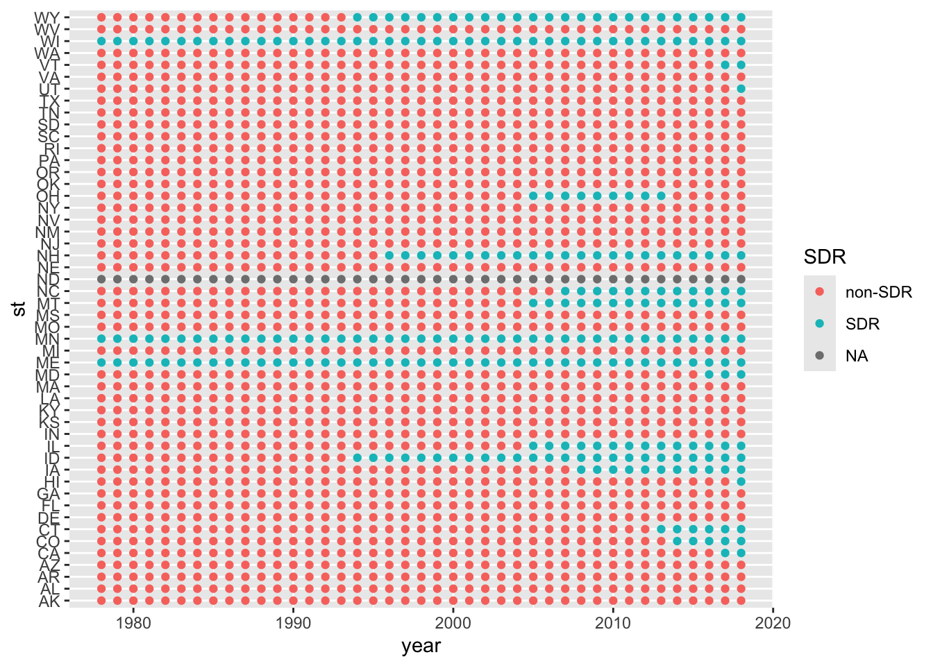
Please answer the following questions:
How many states had Same Day Registration at some point in time? 19 states
How many states had Same Day Registration in 2018? 18 states had SDR in 2018
Did any states get rid of Same Day Registration? When did they get rid of this policy? Yes, Ohio in 2014
What’s up with North Dakota? North Dakota doesn’t require registration to vote. As per footnote 5, they’re excluded from the main analysis.
Use this code chunk to write any code that might help you answer these questions
# Write code to help you answer the questions above (if needed)
# 19 states had SDR at some point
length(unique(policy_data$state[policy_data$sdr==1]))
[1] 19length(unique(policy_data$state[policy_data$sdr==1 & policy_data$ year == 2018])) [1] 18with(policy_data %>%
filter(state=="Ohio"),
table(year,sdr)) sdr
year 0 1
1970 1 0
1971 1 0
1972 1 0
1973 1 0
1974 1 0
1975 1 0
1976 1 0
1977 1 0
1978 1 0
1979 1 0
1980 1 0
1981 1 0
1982 1 0
1983 1 0
1984 1 0
1985 1 0
1986 1 0
1987 1 0
1988 1 0
1989 1 0
1990 1 0
1991 1 0
1992 1 0
1993 1 0
1994 1 0
1995 1 0
1996 1 0
1997 1 0
1998 1 0
1999 1 0
2000 1 0
2001 1 0
2002 1 0
2003 1 0
2004 1 0
2005 0 1
2006 0 1
2007 0 1
2008 0 1
2009 0 1
2010 0 1
2011 0 1
2012 0 1
2013 0 1
2014 1 0
2015 1 0
2016 1 0
2017 1 0
2018 1 0Figure 2 shows the proportion of people voting by age group in states that did and did not have Same Day Registration.
If we take the average of a binary indicator like dv_voted, we get a proportion, which corresponds to what Grumbach and Hill call the Pr(Voted)
With the cps data, use group_by() and summarize() to calculate the proportion of people voting by age group in states that did and did not have same day registration in the code chunk below.
Save the results to a new object called fig2_df
#  Calculate the proportion of voting by age group and SDR
cps %>%
  group_by(age_group, SDR) %>%
  summarise(
    prop_vote = mean(dv_voted, na.rm=T)
  ) -> fig2_df
fig2_df
# A tibble: 14 × 3
# Groups: age_group [7]
age_group SDR prop_vote
<chr> <chr> <dbl>
1 18-24 SDR 0.386
2 18-24 non-SDR 0.315
3 25-34 SDR 0.509
4 25-34 non-SDR 0.452
5 35-44 SDR 0.604
6 35-44 non-SDR 0.561
7 45-54 SDR 0.658
8 45-54 non-SDR 0.617
9 55-64 SDR 0.705
10 55-64 non-SDR 0.666
11 65+ SDR 0.715
12 65+ non-SDR 0.660
13 <NA> SDR 0
14 <NA> non-SDR 0 Using fig2_df recreate a Figure 2 from the paper:
age_group that are NAggplot()#Recreate Figure 2
fig2_df %>%
filter(!is.na(age_group)) %>%
ggplot(aes(age_group,prop_vote,fill = SDR))+
geom_bar(stat = "identity",
position = "dodge") -> fig2
fig2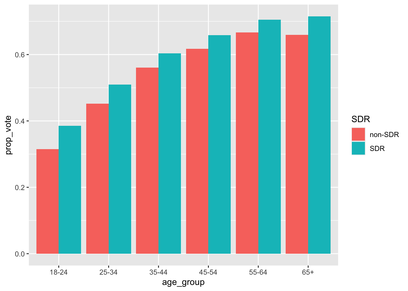
What does Figure 2 tell us? Figure 2 provides initial support for Grumbach and Hill’s general argument. The proportion of people voting in states with SDR is higher than states with out SDR, and this gap is larger among younger age cohorts.
Please take a few moments to complete the class survey for this week.){target=“_blank”} for this week. This one’s a banger.
They also estimate models using both individual and aggregate data, for reasons a bit beyond the scope of this course↩︎
The CPS coding on this is not great and there’s no measure of ethnicity in these data. Forgive the crude indicators, but their necessary to recreate some of Grumbach and Hill’s analysis next week. ↩︎
Note the way the recoding is described in the appendix to the paper is not how it is actually implemented in the replication code in rock_the_reg_replication_code.R. For example, the appendix describes income as ranging from 1 (Under $10k) to 16 ($500k and above), when their code, implemented above produces 32 unique values, in part because the way the CPS asked and coded the income question changed overtime. We’re going to roll with it for now…↩︎